Understanding kinematic concepts requires proficiency in transforming data between representations; differentiation, a core principle in calculus, forms the mathematical basis for converting a position time graph to velocity time graph. The slope of a tangent line at any point on the position time graph, a key attribute, visually represents the instantaneous velocity at that corresponding time. Conversely, MIT OpenCourseWare offers instructional resources that help students master this fundamental conversion, demonstrating a commitment to accessible science education. Therefore, correctly interpreting the graphical relationship between position and velocity provides crucial insights into the motion of an object, impacting fields ranging from engineering to physics, with scientists like Galileo Galilei having established initial theories about motion and time’s relationships.
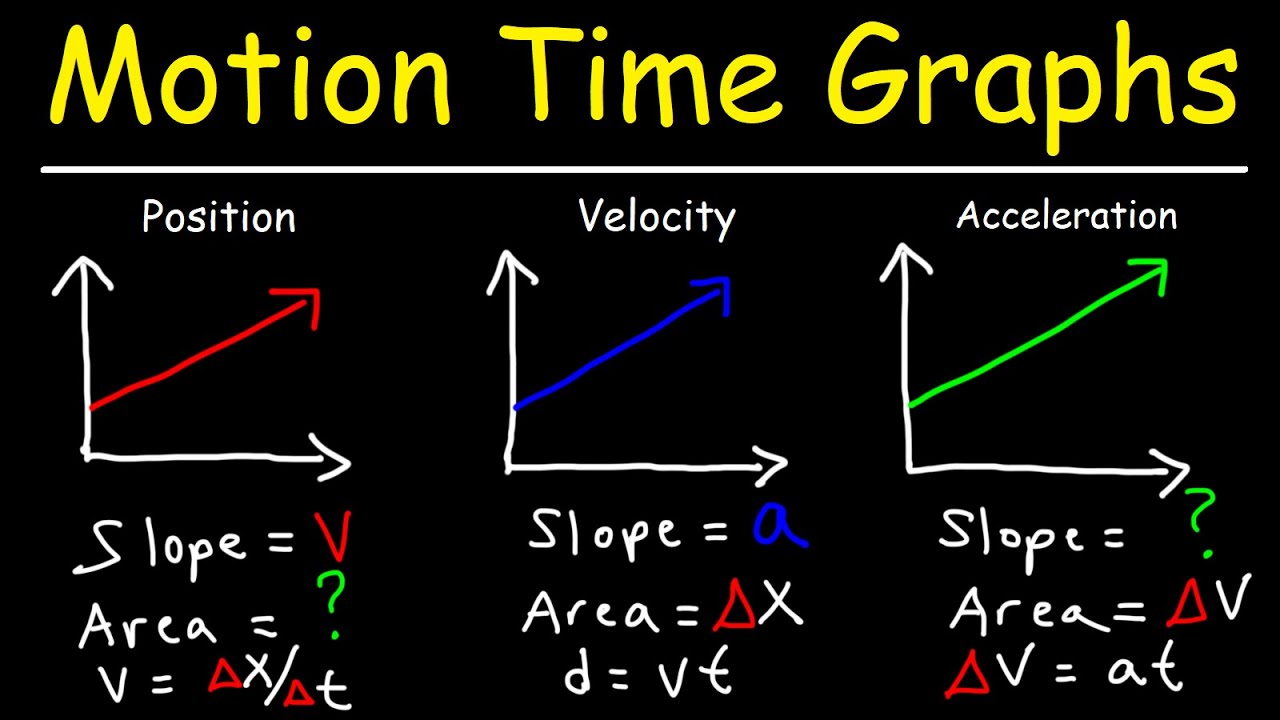
Image taken from the YouTube channel The Organic Chemistry Tutor , from the video titled Velocity Time Graphs, Acceleration & Position Time Graphs – Physics .
Unveiling the Connection Between Position and Velocity Graphs
Position-Time and Velocity-Time graphs are fundamental tools in the study of kinematics, providing a visual representation of an object’s motion over time. These graphs allow us to analyze and interpret how an object’s position and velocity change, offering valuable insights into its movement.
Defining Position-Time and Velocity-Time Graphs
A Position-Time graph plots the position of an object on the y-axis against time on the x-axis. It illustrates where an object is located at any given moment. The shape of the graph reveals whether the object is at rest, moving at a constant speed, or accelerating.
Conversely, a Velocity-Time graph plots the velocity of an object on the y-axis against time on the x-axis. This graph shows how fast and in what direction an object is moving at any given time. The area under the curve of a velocity-time graph represents the displacement of the object.
The Significance of Their Relationship in Kinematics
Understanding the relationship between Position-Time and Velocity-Time graphs is crucial for a comprehensive grasp of kinematics and motion analysis. These graphs are not isolated entities; they are intimately connected through the concepts of displacement, velocity, and acceleration.
Being able to interpret and convert between these graphs allows us to:
-
Predict future motion based on current trends.
-
Calculate important parameters like displacement and average velocity.
-
Gain a deeper understanding of the underlying physics governing the motion.
Objective: A Guide to Converting Position-Time to Velocity-Time Graphs
This article aims to provide a straightforward and accessible guide for converting a Position-Time graph into a Velocity-Time graph. We will explore the underlying principles and provide a step-by-step methodology that demystifies the conversion process. By mastering this skill, you’ll gain a powerful tool for analyzing and understanding motion in various contexts. The goal is to empower the reader with practical knowledge and skills that can be applied to solving real-world problems in physics and engineering.
Foundational Concepts: Velocity, Slope, and the Language of Motion
Before we delve into the process of converting between position-time and velocity-time graphs, it’s crucial to establish a firm understanding of the underlying principles. These graphs are more than just visual representations; they embody the fundamental relationship between position, velocity, time, and, crucially, the slope of a line. Let’s unpack these foundational concepts.
Defining Velocity in Relation to Position-Time Graphs
Velocity, in its simplest form, is the rate at which an object’s position changes over time. In the context of a position-time graph, this means how quickly the object moves along the y-axis (position) as time progresses along the x-axis.
Velocity, therefore, is intrinsically linked to the changing position of the object.
Time as the Independent Variable
The x-axis of a position-time graph invariably represents time. Time, in this context, is the independent variable; it marches forward consistently, allowing us to observe how the object’s position responds.
Each point on the x-axis represents a specific moment in the object’s journey, providing a chronological anchor for understanding its spatial location.
Understanding Slope as Velocity
The most critical concept in converting between position-time and velocity-time graphs is recognizing that the slope of a position-time graph directly represents the instantaneous velocity of the object.
This is not merely a correlation; it’s a fundamental mathematical relationship.
Slope: Rise Over Run (Δposition/Δtime)
Recall that slope is defined as "rise over run." In the context of a position-time graph, "rise" corresponds to the change in position (Δposition), and "run" corresponds to the change in time (Δtime). Therefore, slope = Δposition/Δtime.
But, Δposition/Δtime is the very definition of average velocity. When we consider infinitesimally small changes in time (approaching zero), we arrive at instantaneous velocity.
Therefore, the slope at any point on a position-time graph tells us the object’s velocity at that precise moment.
The Role of Calculus: Differentiation
For those familiar with calculus, differentiation provides a powerful tool for formally understanding the relationship between position and velocity. Differentiation is the mathematical process of finding the derivative of a function.
In our context, if we have a position function, s(t), that describes the object’s position as a function of time, then the derivative of this function, v(t) = ds/dt, gives us the velocity function.
This velocity function, v(t), tells us the instantaneous velocity of the object at any given time, t.
Displacement vs. Average Velocity
It’s important to distinguish between displacement and average velocity. Displacement is the overall change in position (final position minus initial position), while average velocity is the displacement divided by the total time interval.
Average velocity is equivalent to the slope of the straight line connecting the starting and ending points on a position-time graph. Instantaneous velocity, as we’ve established, is the slope of the tangent line at a specific point.
Step-by-Step Conversion: Decoding the Position-Time Graph
Having established the intimate connection between slope and velocity, we can now move onto the practical process of converting a position-time graph into a velocity-time graph. This conversion requires careful analysis, precise calculations, and a systematic approach to translating visual data into meaningful representations of motion.
Analyzing the Position-Time Graph: Unveiling Motion’s Secrets
The first step in the conversion process involves a thorough analysis of the position-time graph itself. We must identify key features that reveal the nature of the object’s motion.
Identifying Constant Velocity and Acceleration
Straight lines on a position-time graph indicate constant velocity. A straight line means the slope is constant, and as we know, a constant slope signifies a constant velocity. The steeper the line, the greater the velocity.
Curves, on the other hand, signify acceleration or deceleration. The changing slope of a curve reveals that the velocity is not constant but is instead changing over time. An upward curve indicates increasing velocity (acceleration), while a downward curve indicates decreasing velocity (deceleration).
Tangent Lines: Capturing Instantaneous Velocity
For curved sections of the position-time graph, the velocity is constantly changing. To determine the instantaneous velocity at a specific point in time, we draw a tangent line to the curve at that point.
The tangent line represents the slope of the curve at that precise moment, providing us with the velocity at that specific instant. This is a crucial technique for understanding motion when velocity is not constant.
Determining Velocity at Specific Points: From Slope to Value
Once we’ve analyzed the position-time graph, the next step is to calculate the velocity at various points. This involves determining the slope of the graph (or the tangent line to the graph) at those points.
Calculating Slope: The Foundation of Conversion
For straight-line segments, calculating the slope is straightforward: rise over run. Select two points on the line and determine the change in position (Δposition) and the change in time (Δtime) between those points. Divide Δposition by Δtime to obtain the velocity.
For curved sections, we use the tangent lines we previously drew. Calculate the slope of the tangent line, using two points on the line, not the curve itself. This slope represents the instantaneous velocity at the point of tangency.
Instantaneous Velocity: Capturing Motion in a Moment
The concept of instantaneous velocity is critical in understanding motion. It represents the velocity of an object at a specific instant in time, as opposed to the average velocity over an interval.
When working with curves on a position-time graph, we are dealing with instantaneous velocities. Each point on the curve has a unique tangent line, and therefore a unique instantaneous velocity.
Constructing the Velocity-Time Graph: Visualizing Velocity’s Journey
The final step is to construct the velocity-time graph based on the velocity values we’ve calculated.
Plotting Velocity Values: From Data to Graph
Plot the calculated velocity values on a new graph where the x-axis represents time and the y-axis represents velocity. Each point on the new graph corresponds to the velocity of the object at a specific point in time, as determined from the position-time graph.
Connect the points to create a continuous line (or curve) that represents the object’s velocity as a function of time.
Constant Velocity: Horizontal Lines on the Velocity-Time Graph
It is important to remember that constant velocity, represented by a straight line on the position-time graph, will manifest as a horizontal line on the velocity-time graph. The height of the horizontal line corresponds to the constant velocity value. If the object is at rest, the horizontal line will lie on the x-axis (velocity = 0).
Examples and Illustrations: Bringing the Concepts to Life
To solidify the process of converting position-time graphs to velocity-time graphs, let’s examine some concrete examples. These examples will cover both simple, constant-velocity scenarios and more complex cases involving acceleration. By visually representing the transformation, we can gain a deeper intuitive understanding of the relationship between position, velocity, and time.
Simple Linear Motion: A Constant Pace
Consider a scenario where an object moves with a constant velocity. On a position-time graph, this motion is represented by a straight line. The slope of this line is constant, indicating a uniform rate of change in position.
Imagine a runner maintaining a steady pace of 5 meters per second. If we plot their position over time, the graph will be a straight line with a positive slope.
The Position-Time Graph
The position-time graph will show a linear increase in position as time progresses. The steepness of the line directly corresponds to the runner’s velocity. A steeper line indicates a higher velocity.
The Velocity-Time Graph
The corresponding velocity-time graph, in this case, is remarkably simple. It is a horizontal line at the value of 5 m/s. This line signifies that the velocity remains constant over the entire time interval. The area under this horizontal line represents the displacement of the runner.
Accelerated Motion: Changing Speeds
Now, let’s analyze a more complex scenario where an object’s velocity changes over time. This is known as accelerated motion and is represented by a curve on a position-time graph.
Think of a car accelerating from rest. Its velocity starts at zero and increases gradually. This change in velocity is what acceleration is.
The Position-Time Graph
The position-time graph for accelerated motion will no longer be a straight line. Instead, it will exhibit a curve. The curve’s shape reveals how the velocity is changing. An upward curve indicates increasing velocity (positive acceleration), while a downward curve signifies decreasing velocity (negative acceleration or deceleration).
The slope of the tangent line at any point on the curve represents the instantaneous velocity at that particular moment in time.
The Velocity-Time Graph
The corresponding velocity-time graph for accelerated motion will be a non-horizontal line. For constant acceleration, the velocity-time graph will be a straight line with a non-zero slope. The slope of this line represents the object’s acceleration.
For example, if the car accelerates at a constant rate, the velocity-time graph will be a straight line with a positive slope, indicating a linear increase in velocity over time. If the acceleration is not constant, the velocity-time graph will also be curved, reflecting the changing rate of acceleration.
Advanced Considerations: Calculus and Non-Linear Motion
While graphical analysis provides a powerful visual intuition for understanding motion, it can become cumbersome when dealing with highly complex, non-linear motion. For scenarios where acceleration is not constant, or where the position function is described by a complex equation, calculus offers a more precise and efficient tool for converting position-time relationships into velocity-time relationships.
Embracing the Power of Differentiation
Differentiation, a core concept in calculus, provides a direct method for determining the instantaneous rate of change of a function. In the context of kinematics, differentiation allows us to find the velocity function, v(t), from the position function, x(t).
Essentially, the velocity at any given instant is the derivative of the position function with respect to time:
v(t) = dx(t)/dt
Unveiling Velocity Functions Through Calculus
This means that if we have a mathematical expression for an object’s position as a function of time (e.g., x(t) = at³ + bt² + ct + d), we can directly calculate the velocity function by applying the rules of differentiation.
For instance, if x(t) = 3t² + 2t + 1, then v(t) = 6t + 2. This resulting velocity function then enables us to determine the velocity at any specific time ‘t’ by simply substituting the value of ‘t’ into the equation.
Advantages of Calculus in Complex Scenarios
The strength of using calculus becomes particularly apparent when the position-time graph is a complex curve, making it difficult to accurately estimate slopes visually. Differentiation offers a systematic and exact method. This provides us with the instantaneous velocity at any moment.
Practical Implications and Limitations
While calculus offers a powerful tool, it’s crucial to acknowledge that it relies on having a well-defined mathematical function for position. In real-world situations, this may not always be the case.
Experimental data may be discrete and require curve-fitting techniques to approximate a continuous function before differentiation can be applied.
Despite this limitation, the application of calculus in kinematics provides a robust framework for analyzing motion. It allows us to derive velocity and acceleration profiles from complex position functions. In turn, we can model and predict the movement of objects with greater accuracy.
FAQs: Understanding Position to Velocity Graph Conversions
Here are some frequently asked questions about converting a position-time graph to a velocity-time graph to help clarify the concepts.
What exactly does a velocity-time graph tell me?
A velocity-time graph displays how an object’s velocity changes over time. The y-axis represents velocity (speed with direction), and the x-axis represents time. It provides a visual representation of motion beyond just position.
How do I determine velocity from a position-time graph?
Velocity is the rate of change of position. Therefore, you determine velocity at any point on a position-time graph by finding the slope of the line at that point. A steeper slope indicates a higher velocity.
What does a horizontal line on a position-time graph mean on the corresponding velocity-time graph?
A horizontal line on a position-time graph indicates the object is not changing position; it’s stationary. Consequently, on the velocity-time graph, this would be represented by a line at velocity = 0.
What happens if the slope of a position time graph is constantly changing?
If the slope of the position time graph is constantly changing, it means the velocity is not constant. This represents acceleration. The corresponding velocity-time graph would show a sloping line (either increasing or decreasing) to represent this change in velocity.
Alright, that’s the gist of turning a position time graph to velocity time graph! Hopefully, this clears things up a bit. Now go out there and graph some motion!