Desmos, a powerful online graphing calculator, provides educators and students alike with intuitive tools. The concept of function notation is fundamental to understanding how Desmos handles different types of graphs. For instance, you can use Desmos to explore the intricacies of desmos how to graph piecewise functions, visually representing mathematical relationships. Khan Academy offers supplemental learning resources that can further clarify these concepts. So, are you ready to dive in and learn desmos how to graph piecewise?
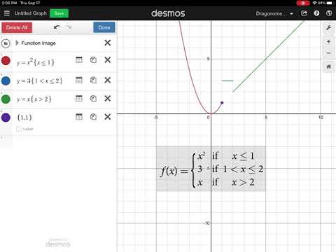
Image taken from the YouTube channel Dragonometry , from the video titled Graphing Piecewise Functions with Desmos .
Graphing Piecewise Functions with Desmos: A Visual Guide
Desmos is a free, powerful, and user-friendly online graphing calculator that has revolutionized how students and educators visualize mathematical concepts. Its intuitive interface and dynamic capabilities make it an ideal tool for exploring various functions, including the often-challenging piecewise functions.
Understanding Piecewise Functions
Piecewise functions are defined by multiple sub-functions, each applicable over a specific interval of the domain.
Instead of a single equation governing the entire input range, a piecewise function uses different equations for different parts of the x-axis. This makes them incredibly useful for modeling real-world situations where different rules apply under different circumstances.
Why are Piecewise Functions Important?
Piecewise functions are essential because they accurately model situations where a single formula cannot describe the relationship between variables across the entire domain. They are crucial in many areas of mathematics, science, and engineering. Their flexibility makes them applicable to a wide array of scenarios.
Article Goal and Purpose
This article aims to provide a clear, step-by-step guide on how to graph piecewise functions using Desmos. We will explore the necessary syntax, techniques for defining domain restrictions, and methods for accurately representing both continuous and discontinuous functions. By the end of this guide, you will be equipped with the skills to confidently visualize and analyze piecewise functions in Desmos.
Understanding Piecewise Functions: Definition and Components
Having established the versatility of Desmos as a graphing tool, it’s crucial to understand the fundamental nature of the functions we aim to visualize: piecewise functions.
Formal Definition of Piecewise Functions
A piecewise function is a function defined by multiple sub-functions, where each sub-function applies to a specific interval within the domain of the overall function.
In simpler terms, it’s a function composed of "pieces," each with its own defining equation and a clearly defined region where that equation holds true.
This contrasts with functions defined by a single formula that applies across their entire domain.
Core Components: Sub-functions
The individual functions that constitute a piecewise function are its core building blocks. These can be linear, quadratic, cubic, exponential, trigonometric, or any other type of function.
Each sub-function dictates the output of the piecewise function within its designated interval. For instance, one piece might be a straight line (f(x) = x + 1) while another is a parabola (f(x) = x²).
Restrictions: Defining the Domain of Each Piece
Perhaps the most defining characteristic of a piecewise function is the restriction placed on each of its sub-functions. These restrictions determine the specific interval along the x-axis where each piece is "active."
Restrictions are typically expressed as inequalities, such as x < 0, 0 ≤ x ≤ 2, or x > 2. These inequalities define the domain for each corresponding sub-function.
The domain restrictions are crucial for accurately defining and graphing the piecewise function. They ensure that only one sub-function is evaluated for any given input x.
Illustrative Examples of Piecewise Functions
Consider the following examples to solidify your understanding:
Example 1: A Simple Two-Part Piecewise Function
f(x) = {

    x + 2,   if x < 0

    x^2,     if x ≥ 0

}
In this example, for any x value less than 0, we use the function x + 2. For any x value greater than or equal to 0, we use the function x².
Example 2: A Three-Part Piecewise Function
g(x) = {

    -x,      if x < -1

    0,       if -1 ≤ x ≤ 1

    x,       if x > 1

}
Here, the function g(x) behaves differently across three distinct intervals. This is a common way to represent absolute value functions.
Example 3: A Piecewise Function with a Constant Segment
h(x) = {

    3,      if x ≤ 2

    x - 1,  if x > 2

}
This example demonstrates how a piecewise function can include constant values for specific intervals. The value of h(x) is always 3 for any x less than or equal to 2.
By understanding the formal definition, core components, and domain restrictions, we lay the groundwork for effectively graphing these functions in Desmos.
Having defined the landscape of piecewise functions, understanding their very nature, it’s time to get hands-on and translate that knowledge into visual representations. Desmos provides an intuitive platform for this, and mastering its syntax unlocks the ability to graph even the most intricate piecewise functions.
Step-by-Step Guide: Graphing Piecewise Functions in Desmos
This section serves as a comprehensive guide, taking you through the process of graphing piecewise functions in Desmos with clear, concise instructions.
We’ll cover the essential syntax, techniques for defining domain restrictions, and strategies for accurately depicting both continuous and discontinuous functions.
Basic Syntax for Piecewise Functions in Desmos
Desmos uses a specific syntax to represent piecewise functions, revolving around curly braces {} and inequalities.
The curly braces are used to enclose the individual function segments along with their corresponding domain restrictions.
Defining Cases with Curly Braces
Each "case" or function segment within the piecewise function is defined within curly braces.
For example, if we have a function that is x + 1 for x < 0 and x^2 for x ≥ 0, the Desmos input will use the following structure:
{x < 0: x + 1, x ≥ 0: x^2}
Specifying the Domain with Inequalities
Within each case, the inequality specifies the domain for that particular piece of the function.
The inequality is placed before the function definition, separated by a colon :.
Desmos supports a full range of inequalities, including <, >, ≤, and ≥, allowing for precise domain definition.
For instance, to define a function that is equal to 5 only when x is equal to 3, you would enter {x=3: 5}.
Inputting Restrictions: Defining the Domain
Accurately defining the domain for each piece is crucial for creating the correct piecewise function graph.
Desmos provides the tools you need to define a variety of restrictions, including open intervals, closed intervals, and even single points.
Using Inequalities to Define Intervals
Inequalities are the primary tool for defining the intervals where each function is valid.
As shown above, you use x < a, x > a, x ≤ a, and x ≥ a to specify the domain for each piece.
Examples of Different Types of Restrictions
- Open Intervals:
x < 2(values less than 2, not including 2). - Closed Intervals:
x ≤ 5(values less than or equal to 5, including 5). - Single Points:
x = 3(only the value 3). - Combined Intervals:
1 < x < 5(values between 1 and 5, not including 1 or 5). - Combining inequalities:
{x<-2: -x-3, -2<=x<=2:x, x>2: -x+3}
Graphing Discontinuous Piecewise Functions
Discontinuous piecewise functions present a unique challenge: accurately representing open and closed intervals at the points of discontinuity.
Desmos can be used to precisely display such functions, visually indicating whether an endpoint is included or excluded from the function.
Representing Open and Closed Intervals Visually
Open intervals (where the endpoint is not included) are represented with open circles, while closed intervals (where the endpoint is included) are represented with closed circles on the graph.
Desmos Syntax for Accurate Interval Notation
To create these circles manually in Desmos, you can graph the point at the discontinuity with appropriate restrictions to define the circle’s fill.
For example, if the function f(x) is x for x < 2 and x + 1 for x ≥ 2, you can explicitly graph the point (2, 2) with the restriction x=2 and style it as an open circle.
Then plot the point (2,3) with the restriction x=2 and style it as a closed circle. This manually adds the visual indicator of open and closed endpoints.
Graphing More Complex Piecewise Functions
Once you’ve mastered the basics, you can tackle more complex piecewise functions with multiple pieces and different function types.
Desmos handles these scenarios with ease, allowing you to visualize intricate mathematical relationships.
Piecewise Functions with Multiple Pieces
Piecewise functions can be defined with any number of "pieces" or sub-functions.
Simply extend the basic syntax, adding more cases within the curly braces, separated by commas.
For instance, a function with three pieces might look like this:
{x < 0: -x, 0 ≤ x ≤ 2: x^2, x > 2: 4}
Combining Different Function Types
The sub-functions within a piecewise function can be of any type: linear, quadratic, exponential, trigonometric, logarithmic, or even combinations thereof.
Desmos allows you to freely mix and match function types within the same piecewise definition.
For instance:
{x < 0: sin(x), 0 ≤ x ≤ π: x/π, x > π: -cos(x)}
This combines a trigonometric function (sin(x) and cos(x)) with a linear function (x/π) within a single piecewise function.
Having mastered the basic syntax and domain restrictions for piecewise functions in Desmos, it’s time to explore some advanced techniques that can significantly enhance your graphing capabilities. These techniques allow for dynamic manipulation, integration with other Desmos features, and efficient troubleshooting, taking your piecewise function graphing to the next level.
Advanced Techniques and Tips for Desmos Piecewise Graphing
Desmos offers functionalities beyond basic graphing that can be leveraged to gain deeper insights into piecewise functions. This includes interactive sliders, integration with data analysis tools, and effective debugging strategies.
Utilizing Sliders for Dynamic Exploration
Sliders in Desmos provide a powerful way to dynamically adjust parameters within your piecewise functions.
This allows you to observe in real-time how changes in the domain, range, or even the function definitions themselves affect the graph.
For example, you can create a slider for the boundary point between two pieces of a function.
As you move the slider, the graph will instantly update, visually demonstrating the impact of shifting the domain restriction.
To implement a slider, simply type a variable (e.g., a) into your piecewise function definition where you want a parameter to be controlled. Desmos will automatically prompt you to create a slider for that variable.
Combining Graphs with Tables, Regressions, and Points
Desmos isn’t just a graphing calculator; it’s a versatile tool for data analysis and visualization.
You can seamlessly integrate your piecewise function graphs with tables of data, statistical regressions, and plotted points.
For instance, you might have a set of data points that you believe can be modeled by a piecewise function.
You can enter these points into a table in Desmos and then define a piecewise function that closely approximates the data.
By adjusting the parameters of the function (perhaps using sliders as described above), you can visually refine the fit between the function and the data.
Furthermore, Desmos allows you to perform regressions on your data.
You can combine a regression with a piecewise function.
This approach can be particularly useful when dealing with real-world data that exhibits different trends across different intervals.
Troubleshooting Common Errors in Desmos Piecewise Functions
Even with careful attention to syntax, errors can occur when graphing piecewise functions in Desmos. Recognizing and addressing these common pitfalls is key to efficient problem-solving.
Syntax Errors
The most frequent errors stem from incorrect syntax, such as missing curly braces or colons.
Carefully review your input, paying close attention to the placement of {} and :. Desmos usually highlights the area where it detects a syntax issue.
Incorrect Domain Definitions
Another common error involves improperly defined domain restrictions. Ensure that your inequalities are correctly specified and that the intervals are non-overlapping, unless you intend for the function to be defined differently at a single point.
For example, x < 2 : f(x), x > 2 : g(x) is valid, but x < 2 : f(x), x > 1 : g(x) may produce unintended results as the domains overlap between 1 < x < 2.
Handling Discontinuities
When graphing discontinuous piecewise functions, it’s crucial to represent open and closed intervals accurately using open and closed circles. Desmos automatically handles this based on the inequalities used.
If you are still having trouble, try explicitly defining two functions. One is for when the condition is met and the other for when it is not, and only display these functions under the appropriate restrictions. This can sometimes prevent unexpected behavior by Desmos.
Having mastered the basic syntax and domain restrictions for piecewise functions in Desmos, it’s time to explore some advanced techniques that can significantly enhance your graphing capabilities. These techniques allow for dynamic manipulation, integration with other Desmos features, and efficient troubleshooting, taking your piecewise function graphing to the next level.
Now, let’s transition from these powerful techniques to the practical applications where piecewise functions shine. The ability to model and visualize real-world scenarios makes understanding piecewise functions even more valuable.
Real-World Examples and Applications of Piecewise Functions
Piecewise functions aren’t just abstract mathematical concepts; they are powerful tools for modeling situations where different rules or formulas apply over different intervals. Graphing these functions offers an invaluable visual aid to understanding their behavior and implications. Let’s explore some common examples and demonstrate how to represent them in Desmos.
Tax Brackets: Visualizing Marginal Tax Rates
Tax systems often use a progressive structure where the tax rate increases as income rises. This is a classic example of a piecewise function. Each "piece" represents a tax bracket with its corresponding tax rate.
For instance, consider a simplified tax system:
- 0% tax on income from $0 to $10,000
- 10% tax on income from $10,001 to $40,000
- 20% tax on income above $40,000
To graph this in Desmos, we can define the tax owed (y) as a function of income (x):
y = {0: 0 < x <= 10000, 0.1(x-10000): 10000 < x <= 40000, 0.1(30000) + 0.2(x-40000): x > 40000}
This Desmos input clearly displays the step-wise increase in tax liability as income crosses bracket thresholds. It visually demonstrates the concept of marginal tax rate – the tax rate applied to each additional dollar earned.
Tiered Pricing: Understanding Volume Discounts
Many businesses use tiered pricing, where the price per unit changes based on the quantity purchased. This is another common application of piecewise functions.
Imagine a scenario with the following pricing structure for a product:
- $10 per unit for the first 10 units
- $8 per unit for the next 20 units (units 11-30)
- $5 per unit for any units beyond 30
In Desmos, we can represent the total cost (y) as a function of the number of units purchased (x):
y = {10x: 0 < x <= 10, 100 + 8(x-10): 10 < x <= 30, 260 + 5(x-30): x > 30}
Graphing this piecewise function reveals the cost savings achieved as the quantity purchased increases, illustrating the concept of volume discounts. It also shows how the slope changes as you move from tier to tier.
Shipping Costs: Flat Fees and Variable Rates
Shipping costs often involve a combination of flat fees and variable rates depending on factors like weight or distance. These scenarios are naturally modeled using piecewise functions.
Consider a shipping company that charges:
- A flat fee of $5 for packages weighing up to 2 pounds
- An additional $2 per pound for each pound over 2 pounds
The Desmos representation of shipping cost (y) as a function of package weight (x) would be:
y = {5: 0 < x <= 2, 5 + 2(x-2): x > 2}
The graph visually shows the discontinuity at x=2, where the cost jumps from the flat fee to the variable rate. This visualization is helpful in understanding the cost implications for different package weights.
Step Functions in Engineering: Control Systems
Step functions, a specific type of piecewise function, are frequently used in engineering to model systems that change state abruptly.
For example, consider a temperature control system that:
- Turns a heater ON (output=1) when the temperature drops below 65 degrees (input < 65).
- Turns the heater OFF (output=0) when the temperature is at or above 65 degrees (input >= 65).
This on/off behavior can be described in Desmos as:
y = {1: x < 65, 0: x >= 65}
This clearly illustrates the instantaneous switch in the system’s state, which is a key characteristic of step functions in control applications.
By graphing these real-world examples, you gain a more intuitive understanding of how piecewise functions can model diverse scenarios and how Desmos can be a powerful tool for visualizing their behavior and implications.
Desmos Piecewise Graphing FAQs
Here are some frequently asked questions about graphing piecewise functions on Desmos, to further clarify the visual guide.
How do I actually create a piecewise function graph in Desmos?
To graph a piecewise function, input the function and its domain restriction together. For example, type y=x{x<0} for the line y=x, but only when x is less than 0. Repeat for each piece of the function. Desmos how to graph piecewise makes it very intuitive.
Why do I need curly braces {} in Desmos when defining a piecewise function?
The curly braces in Desmos act as domain restrictions. They tell Desmos to only graph the function within the specified interval. Without these, Desmos would graph the entire function, defeating the purpose of a piecewise definition. This is how to graph piecewise on desmos correctly.
What happens if the domain intervals in my piecewise function overlap in Desmos?
Desmos will typically prioritize the function defined first. However, it’s best practice to ensure your domain intervals do not overlap. Overlapping intervals can lead to unexpected or ambiguous graphical representations. Avoid overlapping to guarantee Desmos how to graph piecewise works as expected.
How do I show an open circle (hollow point) on the graph where a piece of the function is not defined at the endpoint of an interval?
Desmos doesn’t directly support "open circles." You can approximate it by defining the function very close to, but not at, the endpoint. You could also add a second function that is only a single point. These are some helpful tips on how to graph piecewise on desmos.
Alright, hope that clears up the desmos how to graph piecewise mystery! Now go forth and create some awesome graphs! If you get stuck, just revisit this guide. Happy graphing!